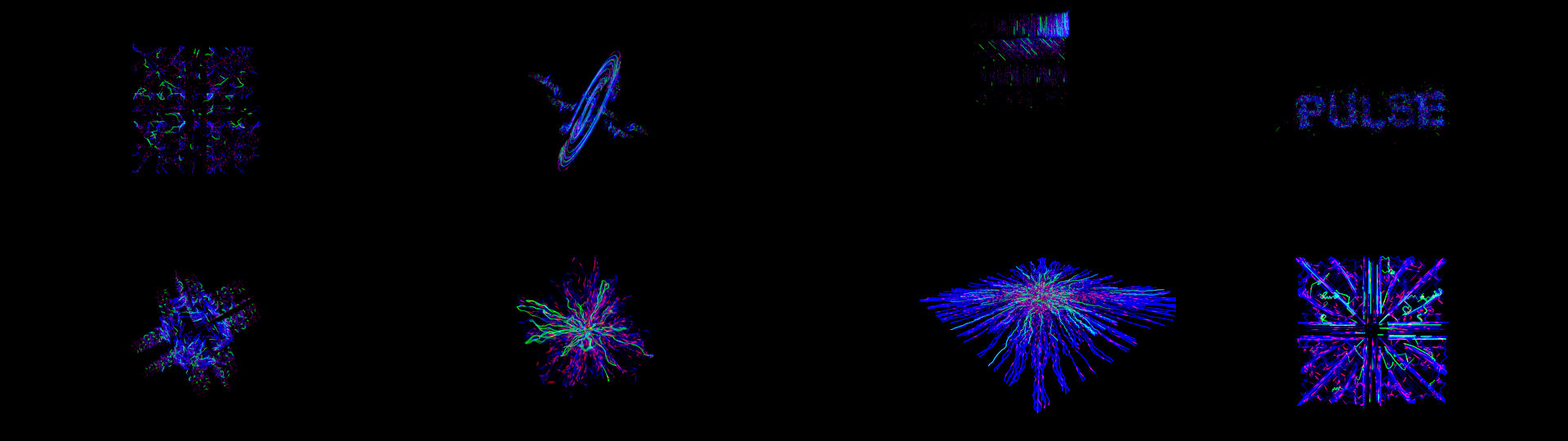
Pulse

Particle vector quantization experiments.

Particle Process

The main technique behind these visuals was a particle setup I came up with last year some time. I found that by driving the velocity of my particles with the position vector of the particle at emission time, quantizing that by some arbitrary value, then running that through a sine function of increasing frequency over time, I could “snap” the particles to predictable but oscillating grid patterns.

As the wavelength grows, you get harmonics running through the values, which randomly steps the velocies back and forward, positive and negative. The wavelength animation was truncated to grow in "pulses" as well, to produce a stepping effect. I then smoothed those curves over time so that there was an easing in and out of each phase of the animation.

There is no keyframing anywhere, this is entirely procedural. Very much a black box setup where tweaking one tiny thing has huge changes.

The raw particle animation driving all of this is super cool all by itself. It’s similar to Cymatics, where patterns are formed by vibration. In the above video, the emission geometry is completely static, and the emission is just random scattering. The square shapes where particles are grouping are actually the quantized 3D coordinates themselves, not polygon faces.

After setting this all up, I could then produce wildly different results by changing the size of the source emitter geometry (which changed the grids that the particles were quantized to), the quantization scaling over time, the velocity scaling, the POP timescale etc. By introducing random noise and wind at various places in the setup, I could introduce some organic elements to the movement and grid constraints while still maintaining the rigid overall shape.

Due to the initial vectors being constrained to grid positions in space, the results could be symmetrical but each would still be unique (which you couldn’t get by just duplicating a slice of the geo and mirroring it on each axis).

I used the particle age to drive the overall shading gradients (@age/(@Frame/24)), then added some randomness with the @id attribute per curve. The emission colours were then varying sine wave frequencies that ran along the lenght of the curve, which grew over time.

Most of the pieces used the normalized age gradient to plot positions in Y space. To create the sagging effect on the wires I just applied an exponent adjustment to the gradient.

The curves were drawn at render time using Redshift, and the different emission attributes were just stored as RGB. Red and green stored the sine waves, blue stored the overall age value.